Compiling ML models to C for fun
NOTE: This post is going to be a compiler post, not a machine learning tutorial, so please treat it as such. Maybe it will still help you understand ML through a compilers lens.
I had a nice chat with my friend Chris recently.
He walked me through the basics of machine learning while I was looking at Andrej Karpathy’s micrograd.
If you are unfamiliar, micrograd is a very small implementation of a scalar-valued neural network (as opposed to vectors or matrices as the computational unit) in pure Python, which uses no libraries.
Micrograd is a combination of a couple of different and complementary parts:
- a little graph-based expression builder and evaluator
- reverse-mode automatic differentiation on that same computation graph
- neural net building blocks for a multi-layer perceptron (MLP)
(If you don’t know what a MLP is, don’t worry too much. This post should give you a bit of background, especially if you are already comfortable with Python. You may want to go through and read and think about the micrograd source code before coming back. And maybe look at this interactive guide too. Or not! Your call. Playing with micrograd helped me a lot. Chris suggested trying to make a network learn XOR.)
Together, these three major components let you write code that looks like this:
from micrograd.nn import MLP
model = MLP(2, [4, 1])
And summon a neural network from thin air.
The thing that got me the first time I read it was that I thought the building blocks were the network. In this library, no. Using a building analogy, they are more like blueprints or scaffolding. With each evaluation of the network, the connective tissue (intermediate computation graph) is constructed anew. In compiler terms, the building blocks are kind of like the front-end and the expression graph is a sort of intermediate representation (IR).
You may be sitting there wondering why I am telling you this. I normally blog about compilers. What’s this?
It’s because once I untangled and understood the three pieces in micrograd, I realized:
- ML models are graphs
- forward and backward passes are graph traversals
- the graph structure does not change over time
- performance is important
Which means… it sounds like a great opportunity for a compiler! This is why projects like PyTorch and TensorFlow have compilers (TorchScript/TorchDynamo/AOT Autograd/PrimTorch/TorchInductor/Glow, XLA, etc). Compiling your model speeds up both training and inference. So this post will not contain anything novel—it’s hopefully a quick sketch of a small example of what the Big Projects do.
We’re going to compile micrograd neural nets into C. In order, we will
- do a brief overview of neural networks
- look at how micrograd does forward and backward passes
- review the chain rule
- learn why micrograd is slow
- write a small compiler
- see micrograd go zoom
Let’s go!
How micrograd does neural networks
First, a bit about multi-layer perceptrons. MLPs are densely connected neural networks where input flows in one direction through the network. As it exists in the upstream repository, micrograd only supports MLPs.
In case visual learning is your thing, here is a small diagram:
In this image, circles represent data (input or intermediate computation
results) and arrows are weights and operations on the data. In this case, the
x, y, and z circles are input data. The arrows going right are
multiplications with weights. The meeting of the arrows represents an addition
(forming a dot product) followed by addition of the bias (kind of like another
weight), all fed into an activation function (in this case ReLU, for
“rectified linear unit”)1. The circles on the right are the results
of the first layer.
Karpathy implements this pretty directly, with each neuron being an instance of
the Neuron class and having a __call__ method do the dot product. After
each dot product is an activation, in this case ReLU, which is equivalent to
max(x, 0). I think the 0 is an arbitrary threshold but I am not certain.
Below is the entire blueprint code for a multilayer perceptron in micrograd
(we’ll come back to the Value class later):
import random
from micrograd.engine import Value

class Module:

    def zero_grad(self):
        for p in self.parameters():
            p.grad = 0

    def parameters(self):
        return []

class Neuron(Module):

    def __init__(self, nin, nonlin=True):
        self.w = [Value(random.uniform(-1,1)) for _ in range(nin)]
        self.b = Value(0)
        self.nonlin = nonlin

    def __call__(self, x):
        act = sum((wi*xi for wi,xi in zip(self.w, x)), self.b)
        return act.relu() if self.nonlin else act

    def parameters(self):
        return self.w + [self.b]

    def __repr__(self):
        return f"{'ReLU' if self.nonlin else 'Linear'}Neuron({len(self.w)})"

class Layer(Module):

    def __init__(self, nin, nout, **kwargs):
        self.neurons = [Neuron(nin, **kwargs) for _ in range(nout)]

    def __call__(self, x):
        out = [n(x) for n in self.neurons]
        return out[0] if len(out) == 1 else out

    def parameters(self):
        return [p for n in self.neurons for p in n.parameters()]

    def __repr__(self):
        return f"Layer of [{', '.join(str(n) for n in self.neurons)}]"

class MLP(Module):

    def __init__(self, nin, nouts):
        sz = [nin] + nouts
        self.layers = [Layer(sz[i], sz[i+1], nonlin=i!=len(nouts)-1) for i in range(len(nouts))]

    def __call__(self, x):
        for layer in self.layers:
            x = layer(x)
        return x

    def parameters(self):
        return [p for layer in self.layers for p in layer.parameters()]

    def __repr__(self):
        return f"MLP of [{', '.join(str(layer) for layer in self.layers)}]"
You can ignore some of the clever coding in MLP.__init__. This ensures that
all of the layers match up end-to-end dimension-wise. It also ensures the last
layer is linear, meaning the neurons do not have an activation function
attached.
But this neural network is not built just with floating point numbers. Instead
Karpathy uses this Value thing. What’s that about?
Intro to the expression builder
I said that one of micrograd’s three components is an expression graph builder.
Using the expression builder looks like a slightly more complicated way of doing math in Python:
>>> from micrograd.engine import Value
>>> a = Value(2)
>>> b = Value(3)
>>> c = Value(4)
>>> d = (a + b) * c
>>> d
Value(data=20, grad=0)
>>>
The Value class even implements all the operator methods like __add__ to
make the process painless and look as much like normal Python math as possible.
But it’s a little different than normal math. It’s different first because it
has this grad field—which we’ll talk more about later—but also because as
it does the math it also builds up an graph (you can kind of think of it as an
abstract syntax tree, or AST).
It’s not visible in the normal string representation, though. Value instances
have a hidden field called _prev that stores the constituent parts that make
up an expression:
>>> d._prev
{Value(data=5, grad=0), Value(data=4, grad=0)}
>>>
They also have a hidden operator field:
>>> d._op
'*'
>>>
This means that we have two operands to the * node d: c (4) and a + b
(5).
I said you could think about it like an AST but it’s not quite an AST because it’s not a tree. It’s expected and normal to have more of a directed acyclic graph (DAG)-like structure.
>>> from micrograd.engine import Value
>>> w = Value(2)
>>> x = 1 + w
>>> y = 3 * w
>>> z = x + y
>>> z
Value(data=9, grad=0)
>>>
Here x and y both use w and then are both used by z, forming a diamond
pattern.
It is assumed that the graph won’t have cycles in it2.
So what does creating the graph look like in code? Well, the Value.__mul__
function, called on the left hand side of an x*y operation3, looks
like this:
class Value:
    # ...
    def __mul__(self, other):
        # create a transient value if the right hand side is a constant int or
        # float, like v * 3
        other = other if isinstance(other, Value) else Value(other)
        # pass in new data, children, and operation
        out = Value(self.data * other.data, (self, other), '*')
        # ... we'll come back to this hidden part later ...
        return out
The children tuple (self, other) are the pointers to the other nodes in the
graph.
But why do we have these expression graphs? Why not just use math? Who cares about all the back pointers?
Let’s talk about grad(ient)
Training a neural network is a process of shaping your function (the neural network) over time to output the results you want. Inside your function are a bunch of coefficients (“weights”) which get iteratively adjusted during training.
The standard training process involves your neural network structure and also
another function that tells you how far off your output is from some expected
value (a “loss function”). A simple example of a loss function is
loss(actual, expected) = (expected - actual)**2 (where ** is exponentiation
in Python). If you use this particular function across multiple inputs at a
time, it’s called Mean Squared Error (MSE)4.
If you are trying to get some expected output, you want to minimize the value of your loss function as much as possible. In order to minimze your loss, you have to update the weights.
To figure out which weights to update and by how much, you need to know how much each weight contributes to the final loss. Not every weight is equal; some have significantly more impact than others.
The question “how much did this weight contribute to the loss this round” is
answered by the value of the grad (gradient) of that weight—the first
derivative—the slope at a point. For example, in y = mx + b, the equation
that describes a line, the derivative with respect to x is m, because the
value of x is scaled by m (and b is a constant).
To compute the grad, you need to traverse backwards from the loss5 to do something called reverse mode automatic differentiation (reverse mode AD). This sounds scary. Every article online about it has scary notation and squiggly lines. But it’s pretty okay, actually, so keep on reading.
Fortunately for us, reverse mode AD, like evaluating an AST top to bottom, it is a graph traversal with some local state. If you can write a tree-walking interpreter, you can do reverse mode automatic differentiation.
Reverse mode AD and backpropagation
Instead of building up a parallel graph of derivatives (a sort of “dual” to the
normal expression graph), reverse mode AD computes local derivatives at each
node in the grad (gradient) field. Then you can propagate these gradients
backward through the graph from the loss all the way to the
weights—backpropagation.
But how do you compose all those local derivatives? There’s no way it’s simple, right? Taking derivatives of big math expressions is scary…
It turns out, calculus already has the answer in something called the chain rule.
The chain rule
I am not going to pretend that I am a math person. Aside from what I re-learned in the last couple of weeks, I only vaguely remember the chain rule from 10 years ago. Most of what I remember is my friend Julia figuring it out instantaneously and wondering why I didn’t get it yet. That’s about it. So please look elsewhere for details if this section doesn’t do it for you. I won’t be offended.
A quick overview
The chain rule tells you how to compute derivatives of function composition.
Using the example from Wikipedia, if you have some function h(x) = f(g(x)),
then h'(x) = f'(g(x)) * g'(x) (where f' and h' and g' are the
derivatives of f and h and g, respectively). This rule is nice, because
you don’t need to do anything tricky when you start composing functions, as
long as you understand how to take the derivative of each of the component
parts.
For example, if you have sin(x**2), you only need to know the derivative of
the component functions x**2 (it’s 2*x) and sin(x) (it’s cos(x)) to
find out the answer: cos(x**2) * 2x.
To take a look at the proof of this and also practice a bit, take a look at this short slide deck (PDF) from Auburn University. Their course page table of contents has more slide decks6.
Also make sure to check out the list of differentiation rules on Wikipedia.
It turns out that the chain rule comes in handy for taking derivatives of potentially enormous expression graphs. Nobody needs to sit down and work out how to take the derivative of your huge and no doubt overly complex function… you just have your building blocks that you already understand, and they are composed.
So let’s apply the chain rule to expression graphs.
Applying this to the graph
We’ll start with one Value node at a time. For a given node, we can do one
step of the chain rule (in pseudocode):
# pseudocode
def backward(node):
    for child in node._prev:
        child.grad += derivative_wrt_child(child) * node.grad
Where wrt means “with respect to”. It’s important that we take the derivative
of each child with respect to the child.
Instead of just setting child.grad, we are increasing it for two reasons:
- one child may be shared with other parents, in which case it affects both
- batching, but that’s not important right now
To make this more concrete, let’s take a look at Karpathy’s implementation of
the derivative of *, for example. In math, if you have f(x,y) = x*y, then
f'(x, y) = 1*y (with respect to x) and f'(x, y) = x*1 (with respect to
y). In code, that looks like:
class Value:
    # ...
    def __mul__(self, other):
        other = other if isinstance(other, Value) else Value(other)
        out = Value(self.data * other.data, (self, other), '*')

        # The missing snippet from earlier!
        def _backward():
            self.grad += other.data * out.grad
            other.grad += self.data * out.grad
        out._backward = _backward

        return out
This means that for each of the children, we will use the other child’s data
and (because of the chain rule) multiply it by the parent expression’s grad.
That is, self’s grad (the left hand side) is adjusted using other’s data
(the right hand side) and vice versa. See what a nice translation of the math
that is? Get the derivative, apply the chain rule, add to the child’s grad.
Now we have a function to do one derivative step for one operation node, but we need to do the whole graph.
But traversing a graph is not as simple as traversing a tree. You need to avoid
visiting a node more than once and also guarantee that you visit child nodes
before parent nodes (in forward mode) or parent nodes before children nodes (in
reverse mode). The tricky thing is that while we don’t visit a node more than
once, visiting updates the node’s children (not the node itself), and nodes may
share children, so children’s grads may be updated multiple times. This is
expected and normal!
For that reason, we have topological sort.
Topological sort and graph transformations
A topological sort on a graph is an order where children are always visited before their parents. In general this only works if the graph does not have cycles, but—thankfully—we already assume above that the graph does not have cycles.
Here is a sample topological sort on the Value graph. It uses the nested
function build_topo for terseness, but that is not strictly necessary.
class Value:
    # ...
    def topo(self):
        # modified from Value.backward, which builds a topological sort
        # internally
        topo = []
        visited = set()
        def build_topo(v):
            if v not in visited:
                visited.add(v)
                for child in v._prev:
                    build_topo(child)
                topo.append(v)
        build_topo(self)
        return topo
To get a feel for how this works, we can do a topological sort of a very simple
expression graph, 1*2.
>>> from micrograd.engine import Value
>>> x = Value(1)
>>> y = Value(2)
>>> z = x * y
>>> z.topo()
[Value(data=1, grad=0), Value(data=2, grad=0), Value(data=3, grad=0)]
>>>
The topological sort says that in order to calculate the value 3, we must
first calculate the values 1 and 2. It doesn’t matter in what order we do
1 and 2, but they both have to come before 3.
Now that we have a way to get a graph traversal order, we can start doing some backpropagation.
Applying this to backpropagation
If we take what we know now about the chain rule and topological sort, we can
do backpropagation on the graph. Below is the code straight from micrograd. It
first builds a topological sort and then operates on it in reverse, applying
the chain rule to each Value one at a time.
class Value:
    # ...
    def backward(self):

        # topological order all of the children in the graph
        topo = []
        visited = set()
        def build_topo(v):
            if v not in visited:
                visited.add(v)
                for child in v._prev:
                    build_topo(child)
                topo.append(v)
        build_topo(self)

        # --- the new bit ---
        # go one variable at a time and apply the chain rule to get its gradient
        self.grad = 1
        for v in reversed(topo):
            v._backward()
The Value.backward function is normally called on the result Value of the
loss function.
If you are wondering why we set self.grad to 1 here before doing
backpropagation, take a moment and wonder to yourself. Maybe it’s worth drawing
a picture!
Putting it all together
I am not going to get into the specifics, but here is what a rough sketch of
very simplified training loop might look like for MLP-based classifier for the
MNIST digit recognition
problem. This code is not
runnable as-is. It needs the image loading support code and a loss function.
The hyperparameters (batch size, etc) are completely arbitrary and untuned.
The full training
code
and corresponding engine
modifications
to add exp/log/Max are available in the GitHub repo.
import random
from micrograd.nn import MLP
# ...
NUM_DIGITS = 10
LEARNING_RATE = 0.1
# Each image is 28x28. Hidden layer of width 50. Output 10 digits.
model = MLP(28*28, [50, NUM_DIGITS])
# Pretend there is some kind of function that loads the labeled training images
# into memory.
db = list(images("train-images-idx3-ubyte", "train-labels-idx1-ubyte"))
num_epochs = 100
for epoch in range(num_epochs):
    for image in db:
        # zero grad
        for p in model.parameters():
            p.grad = 0.0
        # forward
        output = model(image.pixels)
        loss = compute_loss(output)
        # backward
        loss.backward()
        # update
        for p in model.parameters():
            p.data -= LEARNING_RATE * p.grad
In this snippet, constructing the MLP (model = MLP(...)) builds a bunch of
Neurons in Layers and initializes some weights as Values, but it does not
construct the graph yet. Only when it is called (as in model(image.pixels))
does it construct the graph and do all of the dot products. Then we construct
more of the graph on top of that when calculating the loss. This is the forward
pass!
Here is a diagram I made to explain “adding loss on top” to someone:
A sketch-like illustration of a model’s computation graph and loss. The model outputs one value, but how do we know how good it is? Well, we feed it into another subgraph—the loss function—which takes in a second input (the expected value) and itself outputs one value. I made this in Excalidraw.
Then we have the backward pass, where we call backward() on the loss, as I
explained above.
Then we adjust all of the weights by their gradients.
And remember to zero your gradients, folks!

This is nice and simple—thank you, Andrej—but is it fast enough to be usable? Let’s find out.
Performance problems
Uh oh, running this with CPython is slow. It looks like computing a forward pass for one image takes about a second. And then we have to do a backward pass, too. And we have to do several epochs of all 60,000 images. That is going to take way too long!
Well, let’s do what everyone always suggests: try with PyPy. Oh neat, a couple images per second. Unfortunately, that is still not fast enough.
By the way, our old project Skybison is way faster than both CPython and PyPy here! What a fun fact. After some profiling, its major performance pain point was function creation (that is a bit slow in Skybison right now), but if you lift the
_backwardinner functions to the top level, the problem goes away. Then it’s very clear that set lookup from topo sort is the slowest bit in the profile. After that it’s garbage collection from all the transientValueobjects.Incidentally, hoisting the inner functions to be top-level functions also massively speeds up PyPy and it becomes faster than Skybison.
If I had to guess, my hypothesis for the pain points for all of the runtimes is:
- recreating the graph with every forward pass, because of excessive allocation
of
Values and all of their_backwardfunctions- there’s also a ton of allocation and iteration overhead with the
zipinNeuron.__call__
- there’s also a ton of allocation and iteration overhead with the
- doing a topological sort with every backward pass, because of the pointer
chasing, function calls, and
set/listallocation and operations - normal Python interpreter overhead
But if I have learned anything at all over the years, instead of optimizing blindly in the dark, we should first measure.
Checking with a profiler
Emery Berger and his team have released an excellent Python profiling tool
called Scalene. To use it, you can
run scalene yourprogram.py instead of python3 progam.py and when it is
finished (or you hit Control-C), a little locally-hosted website will pop up
with profiling information.
I ran Scalene on our little micrograd MNIST and this is what it looks like.
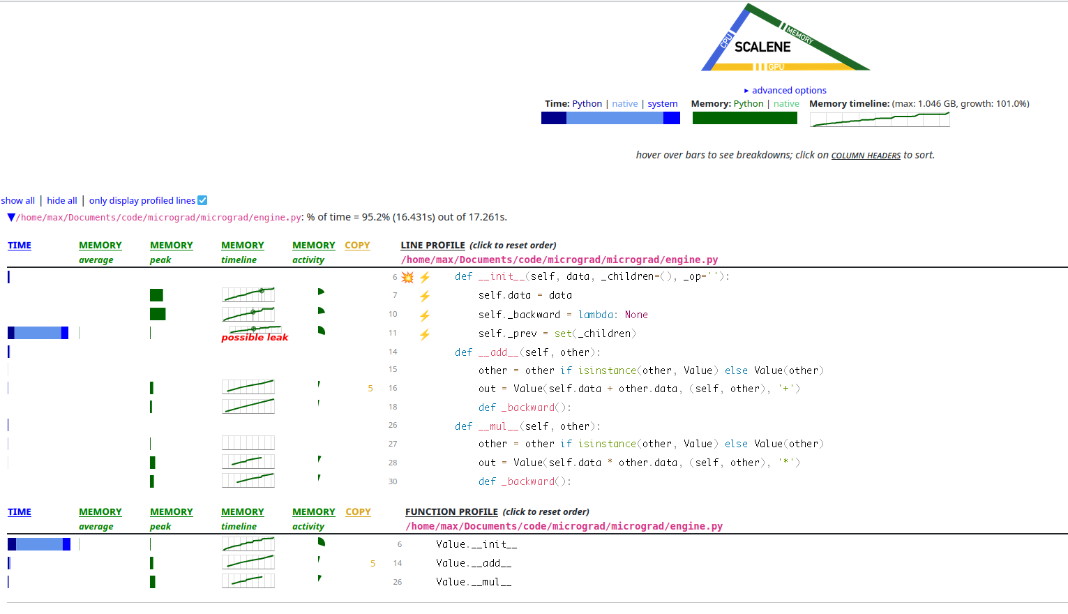
A screenshot of the Scalene profiler’s view of micrograd. It looks
like there is a lot of Value allocation and self._prev being a set could
even be a leak somehow! You can especially see there are a lot of + and *
operations because __add__ and __mul__ allocate a lot.
It looks like in the memory column, the line is going up and to the right,
which is not what we want. It also looks like a huge amount of time is being
spent in creating the set of _prev elements for each Value
If you are old school and don’t trust new profiling tools, you can even confirm
these observations using perf. You’ll need to install the debug symbols for
your Python distribution, probably (in my case it was python3.10-dbg for
Ubuntu) and then you can run perf record python3 yourprogram.py. Here’s what
that view looks like for me (cut off below 0.5%):
Samples: 138K of event 'cpu_core/cycles/', Event count (approx.): 64926188565
Overhead  Command  Shared Object     Symbol
  37.41%  python3  python3.10        [.] gc_collect_main.lto_priv.0
  27.85%  python3  python3.10        [.] deduce_unreachable
   9.91%  python3  python3.10        [.] visit_reachable.lto_priv.0
   3.58%  python3  python3.10        [.] set_traverse.lto_priv.0
   3.29%  python3  python3.10        [.] dict_traverse.lto_priv.0
   2.65%  python3  python3.10        [.] _PyEval_EvalFrameDefault
   2.04%  python3  python3.10        [.] func_traverse.lto_priv.0
   1.67%  python3  python3.10        [.] subtype_traverse.lto_priv.0
   1.16%  python3  python3.10        [.] tupletraverse.lto_priv.0
   0.73%  python3  python3.10        [.] _PyObject_GenericSetAttrWithDict
   0.54%  python3  python3.10        [.] cell_traverse.lto_priv.0
   0.52%  python3  python3.10        [.] insertdict.lto_priv.0
gc_collect_main being 37% of the profile is a massive red flag. Then the
other functions below (deduce_unreachable and all the _traverse functions)
also look GC-related… that means the program is just drowning in allocations.
So Scalene and perf seem to agree.
If you remove the set(_children) and just leave it as a tuple (this seems to
not affect correctness), the profile is a little more spread out.
Another easy enough fix is to add __slots__ to the Value class. Attribute
dicts are the only place I can think of where we are allocating dicts, so maybe
we can take care of that. After adding __slots__, sure enough,
dict_traverse goes away.
Last, we could also try to remove the nested function allocation (as we tried
above for Skybison/PyPy). This will remove func_traverse, too. That’s a
little more work than the previous two micro-optimizations, though.
And none of these little fixes changes the overall architecture of the program, which involves doing so much work to do a little math and a little graph walking7.
So what’s to be done?
Solutions
As I like to say, the best way to make a program faster is to do less. Too much GC? Allocate less. Too much recursion? Topo sort less. Too much overhead? Interpret less. In more detail, my proposed solutions are:
- Re-use the graph structure between inputs. Instead of building a
Valuegraph anew every time, copy in new inputs and propagate them forward and backward. - Since you aren’t changing the graph anymore, no need to re-topo-sort. Keep the ordering around. This helps for both forward and backward passes.
- At the end of the day, the
Valueabstraction does not matter too much. If we know what order to traverse in and are using IEEE-754 doubles, we should compile the topo sort with its operations to C or something more bare-bones8.
This checks out with what we already know about compilers: if you can freeze some of the dynamism in the allowable semantics of a program, you get a performance benefit. Since the graph shape is static, this sounds like a fine idea.
Let’s write a compiler
The goal with this compiler is to write something very small that fits reasonably cleanly into micrograd as it already is—not to re-architect anything.
We could write a compiler to a kind of bytecode. This would get rid of all of the function calls and repeated tree traversals and pointer chasing. It would probably be faster. But unfortunately we would still have an interpreter loop, and that interpreter would be written in Python—would have a lot of overhead.
Instead, we will go further and compile that straight line code to C. The end
goal is to make a Python C extension that we can import and use in place of
the interpreted version of micrograd.
The original version of this project compiled the MLP and Layer and
Neuron classes directly into C, but that unfortunately is not very
extensible: making architectural changes to your model would then require
writing new compilers. It also did not support backpropagation, so it only
helped inference.
For this reason, we are writing compilers for Value graphs. This means
anybody can get a compiler for free as long as their machine learning
architecture uses Values. You need only write an interpreter for it!
Forward
Since we have a topological sort, we might as well use it both forward and
backward. Then we only need to write a compiler that works one Value at a
time. We can drive it like this:
>>> from micrograd.engine import Value
>>> x = Value(1)
>>> y = Value(2)
>>> z = x * y
>>> order = z.topo()
>>> for v in order:
...     print(v.compile())
...
data[1] = 2;
data[0] = 1;
data[2] = data[1]*data[0];
>>>
(Where it is assumed that data is some properly-sized array of doubles that
we will create later.)
Look, there it is! A neat little linearization of the graph. It’s kind of like
the topo sort we saw earlier, but in C code. This strategy works because we
don’t have loops and we don’t have re-definitions of Values. Each value is
set once9. and this code, even with all its memory loads and stores,
should be much faster than pointer chasing and function calls in Python-land.
We could have done this similarly to the interpreted version, where each kind
of operation has its own method (__add__, __mul__, etc), but it’s easier to
present the compiler all in one method. For that reason I am adding a compile
function. See for example the implementation of constant values (op=='') and
multiplication (op=='*'):
class Value:
    # ...
    def var(self):
        return f"data[{self._id}]"

    def set(self, val):
        return f"{self.var()} = {val};"

    def compile(self):
        if self._op in ('weight', 'bias', 'input'):
            # Not calculated; set elsewhere
            return ""
        if self._op == '':
            return self.set(f"{self.data}")
        if self._op == '*':
            c0, c1 = self._prev
            return self.set(f"{c0.var()}*{c1.var()}")
        raise RuntimeError(f"op {self._op} left as an exercise for the reader")
The other operators are not so different. See if you can figure out how to
implement ** or exp, for example. Note that ** requires either storing
additional data or a kind of gross hack.
You may notice that this compilation strategy requires assigning identifiers to
Values. To do that, I have added an _id field that is an auto-incrementing
counter in the __init__ function. The implementation does not matter so much;
just know that every Value object has a unique _id.
My complete compiler implementation for all of the operations is about 40 lines and it even includes some small on-the-fly optimizations. But this compiler does forward passes. What about backward passes? We need to train faster, too. Backward has to be much more complicated, right?
Backward
Actually, it’s about the same complexity. We need only do a line-by-line
translation of the backpropagation functions (all the _backward
implementations).
For example, we can revisit the backpropagation for *. I added some helper
functions to make the code shorter and look more like the interpreted version.
Like the forward version, all the operators are in one method:
backward_compile.
class Value:
    # ...
    def getgrad(self):
        if self._op in ('', 'input'):
            raise RuntimeError("Grad for constants and input data not stored")
        return f"grad[{self._id}]"

    def setgrad(self, val):
        if self._op in ('', 'input'):
            # We don't care about setting gradients for constants or input
            # data.
            return []
        return [f"{self.getgrad()} += {val};"]

    def backward_compile(self):
        if not self._prev:
            assert self._op in ('', 'weight', 'bias', 'input')
            # Nothing to propagate to children.
            assert not self._prev
            return []
        if self._op == '*':
            left, right = self._prev
            return left.setgrad(f"{right.var()}*{self.getgrad()}") +\
                    right.setgrad(f"{left.var()}*{self.getgrad()}")
        raise RuntimeError(f"op {self._op} left as an exercise for the reader")
(Like the forward version, assume for now that grad is some properly-sized
array of doubles that we will create later.)
Let’s see how it works in practice.
>>> x = Value(1, _op='weight')
>>> y = Value(2, _op='weight')
>>> z = x * y
>>> order = z.topo()
>>> for v in order:
...     print(v.backward_compile())
...
[]
[]
['grad[6] += data[7]*grad[8];', 'grad[7] += data[6]*grad[8];']
>>>
Huh, that’s weird. Why is there no backpropagation code for x (grad[6]) and
y (grad[7])? That’s because they don’t have any children of their own;
instead, they are adjusted by their parent node, z (grad[8]). This is what
I meant earlier when I said that visiting a node adjusts the node’s children.
My complete backward pass compiler implementation is about 30 lines! Shorter than the forward pass, even. That’s pretty neat.
You have just finished writing a compiler. Congratulations! Seriously, the
most involved and complicated bit is over. The rest is small details and Python
C-API specifics that you can skip if you like. All we’re missing is update
and set_input and some wrapper code, which are not nearly as interesting.
Update
Once we have done the backward pass (potentially multiple in a row), we need to adjust the weights by their gradients. Code generation for this is a fairly mechanical translation of the Python code into C. For comparison, here is the interpreted version:
def update(model)
    for p in model.parameters():
        p.data -= LEARNING_RATE * p.grad
It loops over the model parameters at run-time and adjusts them. By contrast, the compiled version does the iteration at compile-time and has straight-line subtractions at run-time:
def gen_update(f, model, learning_rate):
    for o in model.parameters():
        assert o._op in ('weight', 'bias'), repr(o._op)
        print(f"data[{o._id}] -= {learning_rate} * {o.getgrad()};", file=f)
# data[0] -= 0.01 * grad[0];
# data[1] -= 0.01 * grad[1];
# data[2] -= 0.01 * grad[2];
# ...
It’s even the same length as the Python equivalent, if you exclude the
assert.
Setting the input
Getting input from Python code into C++ is a little tricky when it’s not simple data types like integers and floats. Ideally our generated ML code would be able to share memory with Python to avoid copying data back and forth, but that wouldn’t be as simple an implementation10, so we’re doing something slightly sillier.
We’re going to have a function set_input that takes its black and white pixel
data in an array of bytes and copies each pixel to its respective slot in the
data array. While this is pretty slow compared to, say, not copying, it is
certainly not the bottleneck in the pipeline.
def gen_set_input(inp):
    result = []
    for idx, o in enumerate(inp):
        result.append(f"data[{o._id}] = buf[{idx}];\n")
    return "".join(result)
In this case, inp is the array of inputs. Unlike with the interpreted version
of micrograd, we are not creating new input Values with every iteration. This
means we have to pre-allocate the range of IDs used for input to and output
from the ML model:
NUM_PIXELS = 28*28
NUM_DIGITS = 10
inp = [Value(0, (), "input") for _ in range(NUM_PIXELS)]
exp = [Value(0, (), "input") for _ in range(NUM_DIGITS)]
out = model(inp)  # create the compile-time Value graph
loss = compute_loss(out, exp)

gen_set_input(inp)
Note that the data or grad fields of each Value node contain garbage data
since inp and exp are arbitrarily chosen. However, the generated C code does
not actually use these Python values. All we care about is the graph structure
represented by the _op and _prev fields.
In order to use this C code from Python, we’ll have to make a Python C extension using the C-API.
A Python C extension
Having a bunch of free-floating code to update data and grad arrays is fun,
and it’s a complete compiler, but it’s not useful yet. We need to wrap that
code in functions (I called them forward, backward, update, and
set_input) and make them accessible to our Python driver program. We don’t
want to have to completely move to C!
Most of this is straightforward (literally print("void forward() {") and so
on), but some of this requires knowledge of Python internals.
For example, here is a snippet of the wrapper code around the forward
function.
PyObject* forward_wrapper(PyObject *module, PyObject *const *args, Py_ssize_t nargs) {
    if (nargs != 2) {
        PyErr_Format(PyExc_TypeError, "expected 2 args: label, pixels");
        return NULL;
    }
    PyObject* label_obj = args[0];
    PyObject* pixels_obj = args[1];
    if (!PyLong_CheckExact(label_obj)) {
        PyErr_Format(PyExc_TypeError, "expected int");
        return NULL;
    }
    if (!PyBytes_CheckExact(pixels_obj)) {
        PyErr_Format(PyExc_TypeError, "expected bytes");
        return NULL;
    }
    if (PyBytes_Size(pixels_obj) != 28*28) {
        PyErr_Format(PyExc_TypeError, "expected bytes of size 28*28");
        return NULL;
    }
    // ...
}
It is an example of a fastcall C-API function, meaning it takes its arguments in an array. We have to register it as such:
static PyMethodDef nn_methods[] = {
    { "forward", (PyCFunction)forward_wrapper, METH_FASTCALL, "doc goes here" },
    // ...
};
And then make a Python-importable module description so that we can create a
module object at import-time:
static struct PyModuleDef nnmodule = {
    PyModuleDef_HEAD_INIT,
    "nn",
    "doc goes here",
    -1,
    nn_methods,
    NULL,
    NULL,
    NULL,
    NULL
};
And then we can create this magic PyInit_nn function. If the Python native
importer finds a module in a .so and it has a PyInit_XYZ function, it will
call it to create the module object.
// Some good keywords are "PEP 384" and "PEP 489".
PyObject* PyInit_nn() {
    PyObject* m = PyState_FindModule(&nnmodule);
    if (m != NULL) {
        return m;
    }
    // ...
    return PyModule_Create(&nnmodule);
}
That’s mostly it! Now we can use all of our hard work in model training and inference.
Did it work? Is it faster?
These are two separate questions and performance doesn’t mean anything if your code produces wrong output.
Correctness
Testing compilers can be tricky. There are a lot of parts and they all have to work on their own and also together. Thankfully in this case, we have a very small compiler with very few basic operations. This makes it not too difficult to write unit tests about the generated C code.
It’s also probably worth having some side-by-side tests on the output numbers of the interpreted and compiled versions of the same code. If they are with some error margin, we can consider the compiler correct. I don’t recommend doing MNIST, though; the interpreted version is too slow and unit tests should be fast. Maybe try XOR.
Thankfully, CPython uses the host system floating point implementation for its
floats, so we get the same numeric behavior as C for no additional effort.
Performance
On my machine, training goes from 1 image per second (interpreted) to >1000 images per second (compiled). This is at least a THOUSAND TIMES speed increase! It comes with an up-front cost, though; you have to compile the C code. If you use TCC, a very fast C compiler, you get pretty reasonable performance. I saw about half second compile times and 45 seconds per epoch. If you use Clang, a much slower C compiler, you get even better performance. Take a look at this handy dandy tradeoff table:
| Compile time (s) | Time per epoch (s) | Speedup | |
| Interpreted | 0 | 60,000 | 1x |
| TCC | 0.5 | 45 | 1333x |
Clang -O0 |
~30 | 30 | 2000x |
Clang -O1 |
~350 | 8 | 7500x |
Either way, this is a pretty big win. I think we did it! Check out the full compiler code and compiler wrapper and training code on GitHub.
Conclusion
Neural networks are represented by static data-flow graphs which are executed in both forward and backward directions. This means they are kind of like tree-walking interpreters. It also means that compiling the tree to a lower-level representation makes the program faster.
On a more serious note: I have traditionally been very uninterested in applying ML because it is oft-used to either harm people (surveillance, recommender systems siloing people, etc) or make software worse (several large companies recently mucked up their chronological feeds, etc).
I learned about machine learning and wrote this post to understand the theory my friends geek out about regularly. I implore you, potential ML practitioner, to use your skills for Good.
Massive thanks to Chris and Bianca for providing significant feedback on this post and to Tom for (naturally) finding and fixing a bug.
More thoughts and further reading
There’s a lot more work to do if you are interested and have the time. I might follow-up on these later. I might not.
Linearizing but still using Python
How much faster can we make the Python version? If we only build the graph once and only topo sort once and just re-set the input every time, do we get faster? I think probably yes. My preliminary numbers show ~100-200x speedup on CPython and ~800x speedup on PyPy. And we didn’t even have to write a compiler!
A Dot operator
If we know we’re doing a dot product in the Neuron class and we know that
operation is going to be fairly common, we might as well have one big Dot
operation instead of a bunch of smaller + and * operations. This lets us
forget about a bunch of the interstitial nodes for both forward and backward
passes (~120k nodes to ~40k nodes) and generate code like:
data[100] = data[0]*data[700]+data[1]*data[701]+data[2]*data[702] // ...
data[101] = data[100]+data[800];
data[102] = relu(data[101]);
This makes our generated code a little easier to reason about. There might be a way to indicate to the compiler, for example, that the dot products for a layer can be vectorized. Or that they can all be done in parallel. This might be a nice speedup.
Unfortunately it does require a change to the neural network code:
diff --git a/micrograd/nn.py b/micrograd/nn.py
--- a/micrograd/nn.py
+++ b/micrograd/nn.py
@@ -1,5 +1,5 @@
 import random
-from micrograd.engine import Value
+from micrograd.engine import Value, Dot

 class Module:

@@ -19,7 +19,7 @@ class Neuron(Module):

     def __call__(self, x):
         assert len(self.w) == len(x), f"input of size {len(x)} with {len(self.w)} weights"
-        act = sum((wi*xi for wi,xi in zip(self.w, x)), self.b)
+        act = Dot(self.w, x)+self.b
         return act.relu() if self.nonlin else act

     def parameters(self):
The code for compiling a Dot node is not that tricky:
def dot(l, r):
    return sum(li.data*ri.data for li,ri in zip(l,r))

class Dot(Value):
    def __init__(self, left_arr, right_arr):
        assert len(left_arr) == len(right_arr)
        assert left_arr
        super().__init__(dot(left_arr, right_arr), tuple(set(left_arr+right_arr)), 'dot')
        self.left_arr = left_arr
        self.right_arr = right_arr

    def compile(self):
        products = (f"{li.var()}*{ri.var()}" for li, ri in zip(self.left_arr, self.right_arr))
        return self.set(f"{'+'.join(products)}")

    def backward_compile(self):
        result = []
        for i in range(len(self.left_arr)):
            result += self.left_arr[i].setgrad(f"{self.right_arr[i].var()}*{self.getgrad()}")
            result += self.right_arr[i].setgrad(f"{self.left_arr[i].var()}*{self.getgrad()}")
        return result
It’s left as an exercise for the reader to think about how backpropagation works. But the results look good:
| Compile time (s) | Time per epoch (s) | Speedup | |
| Interpreted | 0 | 60,000 | 1x |
| TCC | 0.5 | 45 | 1333x |
TCC with Dot |
0.2 | 14 | 4300x |
Clang -O1 |
~379 | 8 | 7500x |
Clang -O1 with Dot |
~330 | 3.5 | 17,000x |
Clang -O2 -march=native with Dot |
~730 | 3 | 20,000x |
Note that we even get better compile times for TCC and Clang -O1 than without
Dot. And it really helps with the preliminary PyPy numbers, bringing those up
to ~3300x. Wow, very nice. Great success.
Compiling for training vs inference
Right now our compilation strategy works for both training and inference. This is great, because it does make both of them faster than before, but it comes with a tradeoff: inference is slightly slower.
If, post training, you freeze the weights and make their immutability known, things get a lot more efficient. Right now we have so many memory loads and stores and it’s hard for the C compiler to prove anything about the properties of the numbers when it is trying to optimize. It probably also prevents use of SIMD instructions. If we can inline the weights as double constants in the generated C code, we can probably get much better machine code.
Scalar-valued is less efficient than tensor-valued
We managed to remove a lot of the overhead for the program we had, but the
overall architecture did not improve much. To do that, we need to move from
scalar-valued to tensor-valued Values.
It’s kind of like programming in assembly (scalar) vs a higher level (tensor)
language. It’s much harder to make optimizations directly on the assembly. If
you have semantically bigger and more descriptive operations in your AST
(matmul, etc), the compiler can better understand what you mean and optimize
that.
It also brings better data locality (matrix is stored densely and in either
row-major or column-major order) and we can get some vectorized math instead of
millions of mulsd.
From what I can tell, optimizing linear algebra IRs is an ongoing area of research.
Using PyPy
PyPy is a JIT compiler for Python, but it also includes a general-purpose programming language called RPython. The neat thing is, if you write an interpreter in RPython, PyPy will turn your interpreter into a tracing JIT compiler. So this brings up some questions:
What if you wrote micrograd in RPython? Would PyPy make an effective JIT out of the tree-walking interpreter… even if it allocated all the AST nodes on the fly? Would it blow the trace length limit?
What if you generated Python code or bytecode? This doesn’t even require
writing the interpreter in RPython, but it does require writing a compiler from
Value graphs to Python (bytecode). Could PyPy compile this effectively?
Follow-up post
I wrote a second post about compiling ML! It’s about automatically vectorizing the scalar IR.
See also Differentiable Programming from Scratch.
-
An activation function is supposed to mimic the behavior of biological neurons when receiving an impulse or something like that. See this blog post for an explanation of why they are necessary. There are other kinds of activation functions, like sigmoid and tanh, but for Math Reasons I Am Too Computer To Understand Right Now, people tend to use ReLU. ↩
-
Apparently even recurrent neural networks (RNNs) are “loop unrolled” meaning they copy and paste the structure in the IR instead of having an actual looping structure. ↩
-
Kind of. This is an oversimplification of Python semantics. If you want to learn more, check out Brett Cannon’s excellent blog post. ↩
-
Another kind of loss function is Cross-Entropy Loss, which is best for (multi-class) classification problems. Adding Cross-Entropy Loss required supporting other fundamental operations on
Valueand in the compiler. ↩ -
There is also forward mode automatic differentiation but I don’t know much about it and haven’t seen it used in my limited search. ↩
-
Daniel Lemire has a great blog post about the myth that performance problems are largely in a few concentrated hotspots. ↩
-
I initially wanted to write the whole pipeline down to machine code by hand. It would still be pretty small, all things considered, but then I would have to do register allocation. Decided to avoid that for now. ↩
-
This makes it SSA form by definition! ↩
-
I think it would be longer, anyway. With our current
dataandgradarray design, we might have to special-case storage for the input data in the compiler—read from a different global variable or something like that. If you use the Python buffer C-API it might not be so bad, actually. Maybe I’ll leave it as an exercise for the reader. ↩